


15’ reading time
A good friend and hedge fund portfolio manager once told me:
‘‘You see that guy? He likes chasing screens.
Once the news is already out, any information asymmetry you perhaps had it’s gone.
You can’t successfully trade old news. Don’t chase the screens’’.
Yes, QT matters. No, QT ≠ mayhem.
Quantitative Tightening is now old news: everybody and their mother are talking about it, and headlines about QT are everywhere.
So, instead of chasing the screens and trading on the news of QT…
Why don’t we have a look at what QT really is and what should you pay attention to?

Without further ado, let’s jump right in!
The QT explainer you were looking for (I hope)
As anticipated here, Central Banks will tighten.
They will try to do it in a gentle way, yes. But they will tighten.
The best definition of ‘‘gentle tightening’’ I can find comes from a speech former ECB president Mario Draghi gave in summer 2017.
If you remember, in 2017 the global economy staged a strong and concerted cyclical recovery - mostly due to the lagged effect of a huge 2016 Chinese credit expansion and some fiscal stimulus in the US.
‘‘As the economy continues to recover, a constant policy stance will become more accommodative, and the central bank can accompany the recovery by adjusting the parameters of its policy instruments – not in order to tighten the policy stance, but to keep it broadly unchanged.’’

Jokes aside, the prospect of 4 hikes plus QT at the same time sounds all but gentle.
So, where is the trick?
The devil is in QT’s details.
Quantitative Tightening is the opposite of QE: Central Banks reduce their balance sheets by eliminating reserves from the system and they force the private sector to rebalance their asset composition from zero-risk, zero-duration reserves (banks) or bank deposits (non-banks) into credit and duration-intensive bonds.
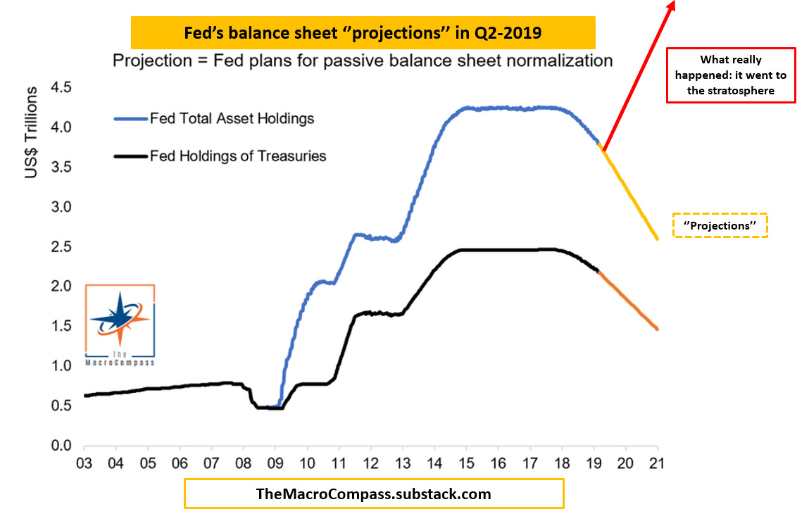
Analysts now expect the Fed to shrink its balance sheet by about $1.5 trillion between mid-2022 and the end of 2023.
Here is what analysts were expecting in Q2-19 (orange) and what really happened (red).
Why is it so complicated to engineer a successful QT, and will Central Banks manage this time around?
Let’s look at the mechanics for a second - I was inspired by this post from The Fed Guy (Joseph Wang): check him out, he’s great!
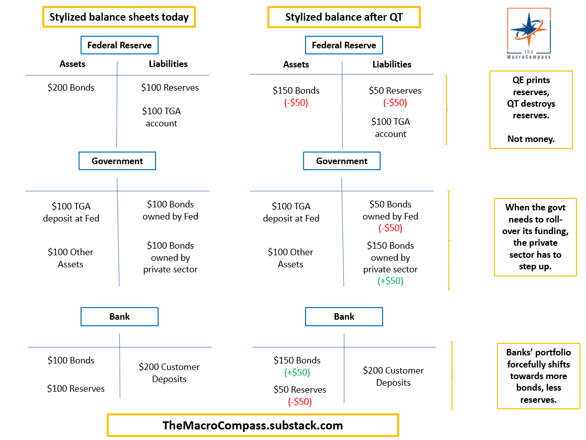
In the example above:
A) The Fed has reduced its balance sheet with a couple of keystrokes; just as it created reserves out of thin air to run QE, now it doesn’t reinvest maturing bonds from its QE portfolio (= performs QT) and therefore destroys reserves;
B) We assumed the government would just roll-over its funding needs: as the Fed isn’t rolling over its bond holdings, the private sector now needs to step up and absorb more of the newly issued securities;
C) The private sector (identified with commercial banks here) has to forcefully change its asset side portfolio composition into owning more bonds and less bank reserves. For a non-bank private entity, the conclusion is similar: it would need to own more bonds, and less bank deposits.
So, what makes running QT so hard?
There are two reasons: the ‘‘cash’’/collateral positive imbalance gets reversed and the QE-driven incentive to move down the risk curve gets incrementally reduced.
To understand why that’s really hard to do, let’s look at what QE does first.
After all, QT is the opposite of QE.
Say you are a pension fund in the Eurozone.
On the asset side of your balance sheet you need bonds to a) offset the duration risk of your long liabilities, b) generate some yield, c) because the regulators say so.
Now, with QE the ECB has been forcefully changing the composition of your portfolio by removing bonds from the system and injecting inert bank deposits.
Here is a stylized example:

Notice: pension funds don’t have access to the ECB, and therefore their default choice would be to deposit money overnight at European commercial banks.
Yes. Unsecured, non-collateralized bank deposits at -58 bps (banks swimming in excess reserves will obviously charge rates below the -50 bps ECB deposit rate for additional deposits, such that they can generate returns able to compensate for balance sheet and leverage ratio costs).
Not a nice proposition.
So, what do they do instead? Reverse repos.
Pension funds would lend away their ‘‘cash’’ (i.e. inert bank deposits) and get back ‘‘collateral’’ (i.e. bonds) in exchange - this way, their overnight unsecured deposit at a commercial bank has turned into a secured, collateralized reverse repo transaction.
As the ECB drains collateral from the market and continuously injects ‘‘cash’’ (bank reserves and inert bank deposits), the positive ‘‘cash’’/ negative collateral imbalance becomes bigger and repo levels become incrementally more expensive - sometimes even returning way less than a risk-free overnight deposit at the Central Bank.
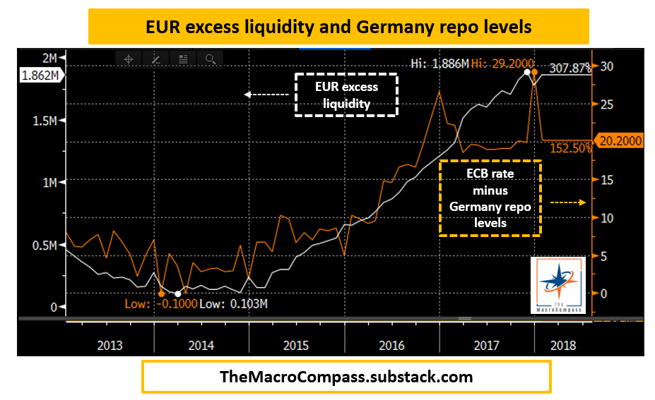
So: more ‘‘cash’’ chasing less and less ‘‘collateral’’ = more expensive repo levels.
Why does it matter?
Repos are used by primary dealers, hedge funds and about any other financial institution to borrow and lend money and securities to each other’s.
When repo rates turn very expensive, borrowing scarce securities to sell them short becomes a pretty expensive exercise - on the other hand, she who owns the shrinking amount of collateral and decides to lend it out gets a nice compensation in return.
This bring us to the QE-driven incentive to move down the risk curve.
The ‘‘abundant cash / scarce collateral’’ imbalance leads to more expensive repo levels, which makes short-selling government bonds more punitive ceteris paribus.
Generally speaking, this new incentive scheme leads to lower volatility: an increasing amount of ‘‘cash’’ chasing a shrinking pool of collateral makes sell-off look like a palatable opportunity to buy. A gravitational force, basically.
On top of that, the private sector now sits on a portfolio much more skewed to zero-yielding, zero-duration reserves than to much needed coupon and risk-bearing bonds.
Time for carry trades.
Below, the % of high-quality liquid assets major American banks chose to allocate to reserves (blue), Treasuries (green) and higher-yielding yet still regulatory-friendly liquid assets (orange and white).
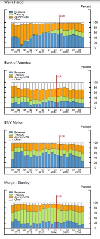
The common trend is for a lower HQLA percentage held in reserves or Treasuries, and more allocated to higher-yielding assets: mortgage backed securities (MBS) and other bonds treated as HQLA under the Liquidity Coverage Ratio (LCR) regulation.
Hint: that’s mostly highly-rated Corporate Bonds.
Carry trades, indeed: less collateral versus more ‘‘cash’’, more expensive repo levels, less volatility = investors move down the risk curve and buy riskier securities.
All clear, so far?
Now, just think that QT delivers the exact opposite effects of QE.
Reserves get removed from the system while the collateral previously bought by Central Banks does not get repurchased once it matures: the ‘‘cash/collateral’’ imbalance starts to revert.
As the private sector is called to marginally absorb more collateral while owning less reserves and inert bank deposits, their marginal appetite to increasingly move down the risk curve reduces ceteris paribus.
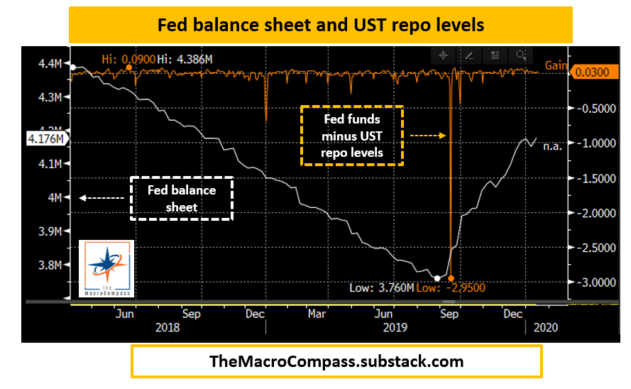
Here is a look at what happened in September 2019, when the Fed had reduced its balance sheet from $4.5 trillion to $3.8 trillion in 2 years.
Conclusion: shall we freak out?
No.
While QT sets the direction of travel to be very different from QE, there are four main pillows the US will be using to engineer a softer landing.

The starting point and the pace of QT: although nobody knows ex-ante what’s the amount of excess liquidity which holds the system comfortably together, reducing the balance sheet from $9 trillion to $7 trillion in a couple of years is unlikely to make everything blow up ceteris paribus.
The standing repo facility (see here): in July 2021, the Fed introduced a permanent repo facility which allows market participants to lend securities at Fed Funds rate plus 25 bps to the Federal Reserve in exchange for cash. While this might not be enough to fully shield the repo market from undue distress, it surely reduces tail risks.
The Treasury issuance strategy: as we discussed, the private sector will be called to absorb more securities (carrying duration and credit risk) while owning less reserves. The Treasury is likely to temporarily shift the issuance pattern towards bills, which carry very little duration and credit risk hence facilitating the private sector’s task.
The RRP release valve: additional bill issuance could be easily absorbed by money market investors, which are today instead placing $1.6 trillion excess liquidity at the Reverse Repo Facility.
In a nutshell: watch the announcement on the pace of QT, the updated Treasury issuance strategy and how repo rates and credit spreads trade.
But don’t panic on QT headlines, please.
If you enjoy my work, please consider clicking on the like button and share the article.
It costs you literally nothing, but it would really make my day!
Are you an institutional investor who likes The Macro Compass and would be interested in a bespoke, pro-to-pro coverage?
Are you looking for any other kind of partnership or collaboration?
Feel free to get in touch at themacrocompass@gmail.com.

See you again on Monday!


The Fed's QT Explained (No, it's Not The End Of The World)